
Project Nahual
The blog
In this blog I will explain my journey on this project and maybe share some other thoughts if they ever come to my mind.
The project
The project is in its first steps and best described by the blog article “On Project Nahual”. Have a look and maybe let you inspire yourself.
Me, myself and I
Who is “I”? I’m Jannik Baumgart. I am from germany, currently working at a medtech company and am a space nerd by heart.
-
First simulations
It has been far too long. I had some very interesting things happening in my life. They were and are very nice. In the last months I have come to work on Nahual a lot more again. I have understood a lot more about the space weather modeling framework (SWMF) and specifically the global magnetosphere (GM) simulation I am mainly using.
A short wrap-up from the past: I want to make a proposal for a satellite, which is able to protect the atmosphere of planet Mars from solar wind, if we ever decide to terraform it. Mars does not have a natural magnetic field as the Earth has. The SWMF allows simulations of the solar wind plasma.
For this article I have simulated a magnetic satellite with 17km diameter and a varying magnetic field strength of 10, 20 and 30T at the Sun-Mars L1 Lagrange point. Everything in this simulation is measured in Mars radii R (3.400km). Every dot represents a cell with data. The dots are colored based on the particle density in each cell. Blue means few particles, red means many particles. We want blue cells around Mars (the single red dot at the center).

0.005R (17km) size 10T magnetic field at 320R (1.088.000km) upstream to Mars. There is a small blue low-density zone behind the position of the satellite. Around it a high-density zone is visible. This is a bow shock forming just as it does on Earth’s magnetic field. There many fast particles are slowed down tremendously. 
0.005R (17km) size 20T magnetic field at 320R (1.088.000km) upstream to Mars. The bow shock gets considerably bigger and the maximum density is higher. The density in a cell near Mars is lower than with 10T. 
0.005R (17km) size 30T magnetic field at 320R (1.088.000km) upstream to Mars. The perturbations of the magnetic field are thousands of kilometers across and stretch over more than a million kilometers. 
0.005R (17km) size 30T magnetic field at 320R (1.088.000km) upstream to Mars. Data view from a cell close to Mars. It is even lower than with 20T. While 17km and 10T are still very huge, seeing the size of the perturbations on an object “just” 17km wide, gives me hope to look for a smaller solution. It is worth noting, that I experienced a lot stronger perturbations on simulations with higher resolution. I use these images to understand the produced simulation data. But since a simulation is solely based on my input parameters, they are probably still quite some steps away from showing a realistic simulation.
On earlier simulations as well as this simulation I found, that the perturbations tend to weaken downstream. The images show a very strong reduction in density close to the magnetic field, but not very far behind. Due to this, I revised the original idea of putting something at the L1-Lagrange of Sun and Mars. With a bit of help of an AI I thought about alternative solutions. Currently I simulate with 10R (34.000km) distance to the planet. The strategy would be three or more identical satellites with excentric sun-synchronous orbits with its apogee (highest point) facing the sun. Sun-synchronous orbits wander over the year, due to some planets not being perfect spheres, and stay between Sun and planet. However, since it only stays there for a given amount of time before going into the shadow of the planet, more satellites are required. As an advantage, the orbits are easier to navigate than Lagrange orbits and are reasonably stable against the expected solar wind magnetic pressure, which is small but not negligible. The force on the satellites at the “day-side” of this eccentric orbit is less influential as the force negates itself over time or exerts tangential at apogee.
There are a lot of questions remaining, that need an answer. And as it is with science, when you solve one, you get more new questions. They are not solved by plasma simulations alone, but I will follow the main route for the moment. Some of the questions boggling me:
– Is a low-pressure low-density zone in this simulation sufficient to protect an atmosphere? Or are there also other effects at play?
– What magnet size will be reasonably doable? I will see whether I can push down to below 1km construction diameter. Is a magnet that small in size able to create the needed plasma perturbations?
– Is a shield necessary in the first place? While the solar wind degrades atmospheres, this might take millions of years to do so. Maybe terraforming the Mars wouldn’t even need it, as the erosion is neglegible anyway.
I am already advancing further than in this blog post, but I needed to start somewhere again. So there will be more to share eventually. Looking forward.Direct link to article and comments: https://nahual.eu/first-simulations/
Download files: https://nahual.eu/wp-content/uploads/2026/05/First-simulations.zip

17km -20Tfront view – just for data gazing 
17km 30T front view inside – just for data gazing
-
On how the work actually looks
I want to share some progress on my work with the Space Weather Modeling Framework. To get you on board again, I try to simulate a solar magnetic shield for Mars. It is best explained in the blog article On Project Nahual. Somewhere later in time, I got prominent support and discovered the Space Weather Modeling Framework (SWMF). For that, see On plans.
In the meantime, I got a lot more comfortable with the usage of the SWMF. I use the software to simulate planetary magnetic fields (like Earths magnetic field) and their interaction with solar wind. This way, I get a better understanding about how these magnetic fields behave and what influences them. But to get away from this most theoretical level (and stay on a still very theoretical level), I first want to share, how this work actually looks.
The SWMF is capable of many things and it has a specific module called “global magnetosphere”, which is exactly what I need and use. After an installation in a Linux distribution inside Windows, I can start a modelling run by providing a parameter file and giving a start command. This is now quite comfortable. However, it took me quite a while to get the inputs to the parameter file reliably working. I added a video to show the workflow.
My SWMF workflow – Linux subsystem for windows is on the left and controls the SWMF, on the right is the parameter file. After a completed run, a post-processing script produces readable data, from which I produce images with a python script of most questionable quality. With this setup in place, I can always directly see the outcome of changes in the parameter file. My currently latest advancement is the modeling of two separate magnetic fields, the Earths and an arbitrary second object. In later stages, this would be the Mars without a magnetic field and a small object with magnetic field of not yet known specifications.
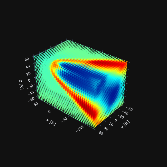
This was my first successful image for two separate magnetic fields. The color of the dots represents the density, the size represents pressure. With this representation, you can perfectly see the red high-density bow shock line and its low density region forming behind. With this “#SECONDBODY”-feature learned, I started to look at some simulations closer to my use case. While I could just change to Mars as a chosen first object, it would not interact with the solar wind on a planetary scale, so it does not give me additional information (and looks less interesting). The second interesting change for my use case is the actual distance of things. The “global magnetosphere” model uses the planet radius as distance unit. I understood this only pretty recently as I tried to get the distance of things right. While it may seem counterintuitive to have a distance measurement and a grid which is completely different for each planet, it saves computational resources to normalize everything to this. At least that is how I understood the design choice explanation.
This also means, a grid, which is from -60 to 60 [R], actually spreads over 120 Earth radii with only 20-something dots (depends on the refinement parameters). So there easily fits an Earth or two between each of the simulation dots. The Earth has a mean radius of 6.137 km. It is possible to get better resolution, but of course, this costs computing power and I need to learn, how the refinement parameters work. To achieve the distance of Mars and its L1 Lagrange point, I would need to place the second object at around 140 Earth radii. I tried this, but I got several problems, with the size and uniformity of the grid as well as even this level of refinement. This is nothing, which cannot be solved by some tinkering with the parameters, however to get something working for this milestone, I settled for 80 Earth radii distance, because I got it to work way easier. For Earth, this is a distance of around 500000 km. For reference, the moon is at 384400 km and the ISS is at around 420 km. Actually calculating the distances always gives me a feeling for the actual size of even our closest neighborhood.
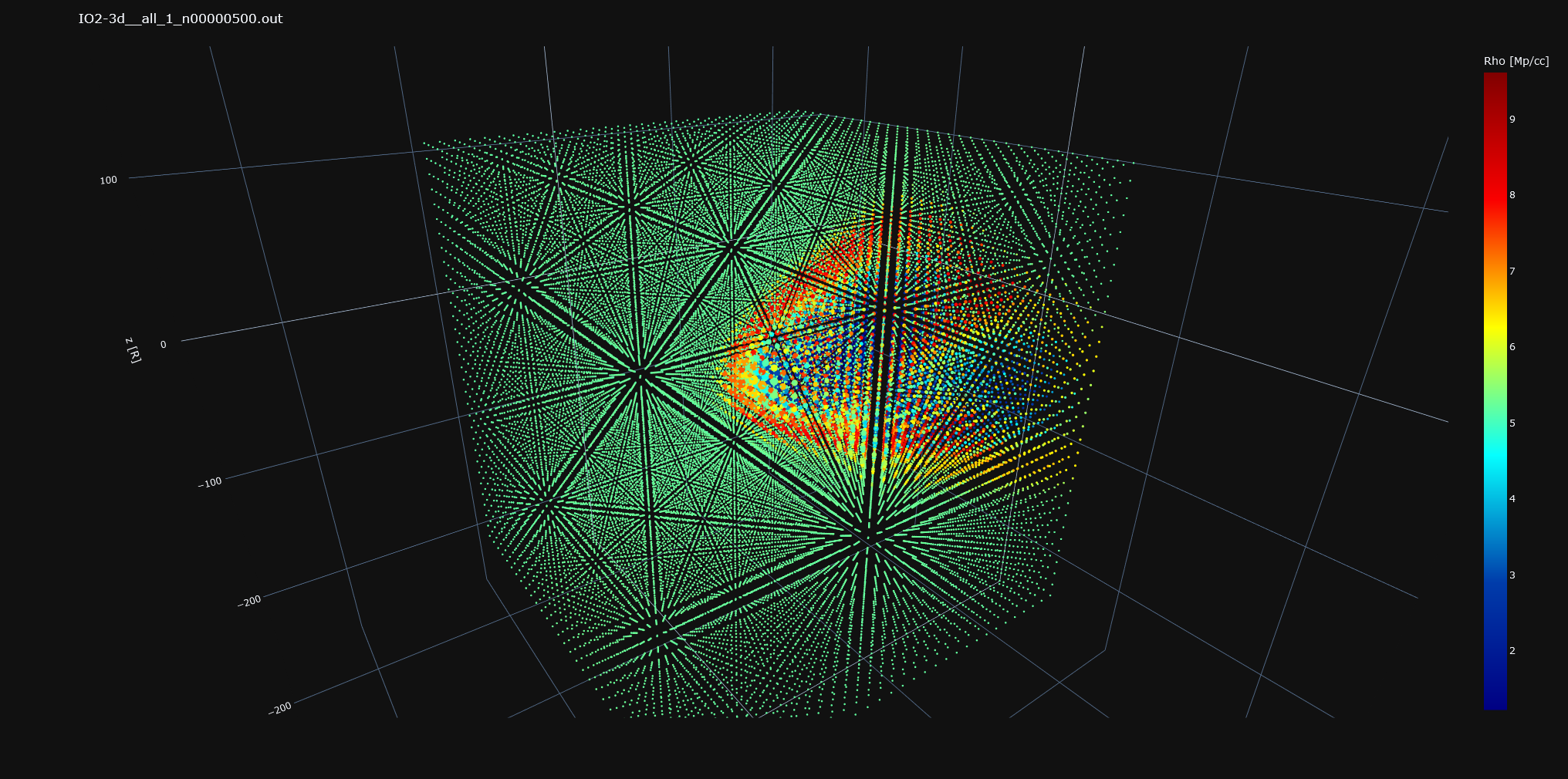
Image of the simulation with 80 Earth radii distance between two bodies on the Y-axis. Another target or idea for this milestone was to improve the images by reducing less useful data. It obstructs the view and the python imaging library Plotly also has some soft limitations on how many dots it can produce. When working with the WSA-ENLIL model, the size of the less interesting dots conveniently was small enough, however for the SWMF and my parameters, this is not the case. Additionally, the most interesting dots are the ones with very high or very low values. As a cheap solution, I just not printed dots with the median density +- 5%.
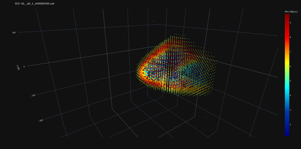
Image of the 80 Earth radii simulation with only data points printed, which are not the median +-5% density. Will be referred to as “relevant grid”. 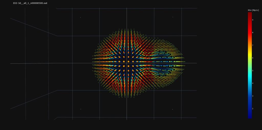
Image of the 80 Earth radii simulation with relevant grid from the front. While a 2D representation might be more useful or clearer for a website, I am very happy for the 3D images, as they allow for a better understanding of the data and a more direct way to spot errors, as explained in my first blog post On graphing the stars.
Now for a last learning with this feature, I wanted to move the second body between Sun and Earth. See the following top-view images.
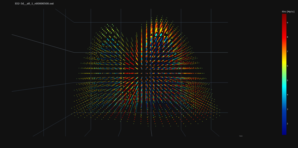
Image of the 80 Earth radii simulation with relevant grid from the top. 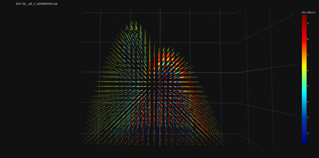
Second body moved on X-Y-plane with 80 Earth radii distance with relevant grid from the top. 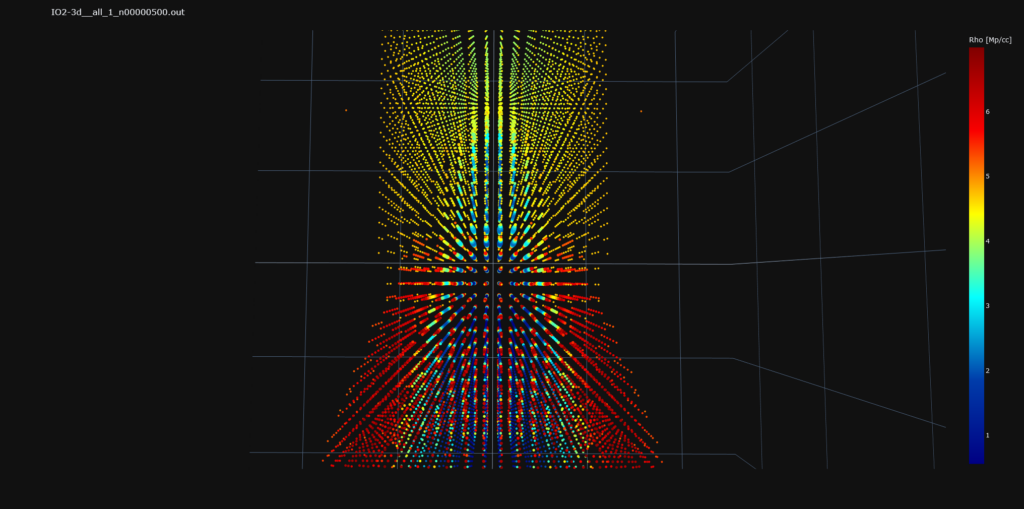
Second body with 80 Earth radii distance on X-axis with relevant grid from the top. With moving the second body from the Y axis to the X Axis in Front of the Earth, I get this simulation artifact, where no bow shock can be found for the second body in front of the Earth. I suspect, the “perturbation” of the magnetic field are too close to the connection to the ambient medium, which feeds the “global magnetosphere” model. I experienced a similar issue, when I moved the X-axis simulation border too close to the Earth at an earlier testing. I suspect to solve or work around this problem and increase my simulation size and resolution, but for the moment I am quite happy, to get a reliable output and gaining a lot of knowledge about the SWMF as well as space weather itself.
I currently plan to do a bit of paper reading to feed my learnings of space weather with technical Know-how. But plans change as the weather does. And in the meantime, life happens to be complicated. Beautiful and complicated. See you around.
All pictures and content to download: On-how-the-work-actually-looks.zip
Direct link to post and comments: https://nahual.eu/on-how-the-work-actually-looks/
-
On plans
So, sometimes life goes not exactly like you plan it to be. On closer look, it rarely goes as expected. Depending on how you feel about live and curiosity, this is usually a good thing. In the last blog post, I told you about the plans I had with the WSA-ENLIL model. Spoiler alert: plans changed.
In the first steps of Project Nahual, I familiarized myself with solar wind with the help of the WSA-ENLIL model. To start an actual simulation of an artificial Martian magnetic shield, I tried to get my hands on the source code of this WSA-ENLIL model. I dug through the internet without success. The only option would be to request a run with specific parameters, though defining such specific parameters (e.g. ones who actually weren’t intended by the creator) is impossible without an extensive documentation or the source code. I found this option at the Community coordinated modeling center (CCMC) run by NASA. https://ccmc.gsfc.nasa.gov/
In an old school attempt, I wrote an email describing my issue to the CCMC model hosts. And someone answered! Someone from NASA wrote me an email. This absolutely made my week and is still absolutely awesome. Unfortunately, they could not help me with my request of the WSA-ENLIL model. It is not open source, only model runs can be requested. But they told me about an alternative, the Space Weather Modeling Framework (SWMF) created and maintained openly with the University of Michigan. Welp. So now they not only answered, they also supported me. And the SWMF apparently is an absolutely powerful tool. The documentation is insanely good and I immediately had the feeling, that it will make my simulation efforts a whole lot easier. I’m currently doing baby steps with a program designed for super computers by absolute experts in their field.
It took me quite a while to get the model up and running on my system. This is also a work in progress for me, since the options are basically unlimited. However, to again show you something I had the model produce 3D-data of the earth’s magnetosphere. Enjoy, but don’t use it for any scientific purposes. I am by no means sure, I gave the model physically authentic input.


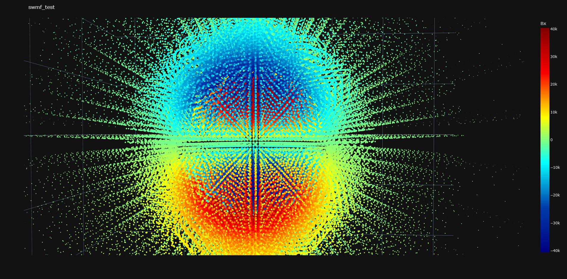
Geomagnetic 3D data from the SWMF So after releasing the last blog post, I would’ve never guessed, where my project would lead me. You can be sure, that I love this path, though. My plan for the next one is a bit vague. Since in the meantime some people of the real life told me “I have no idea, what you are doing there”, I’d like to give some insight about how using this model actually looks. But we will see about the future.
Direct link to article and comments: https://nahual.eu/on-plans/